Python notebooks as dataflow graphs: reactive, reproducible, and reusable

This blog is adapted from our talk at PyCon 2025. marimo is free and open source, available on GitHub. For a free online experience with link sharing, try molab.
marimo is a new kind of open-source Python notebook. While traditional notebooks are just REPLs, marimo notebooks are Python programs represented as dataflow graphs. This intermediate representation lets marimo blend the best parts of interactive computing with the reproducibility and reusability of Python software: every marimo notebook works as a reactive notebook for Python (and SQL) that keeps code and outputs in sync (run a cell and marimo knows which other cells to run), an executable script and a Python module, and an interactive web app.
In this blog post, we motivate the need for a new kind of notebook, explain how and why marimo represents notebooks as dataflow graphs, present design decisions we made to help users adapt to dataflow programming, discuss our implementation, and show several examples of how marimo uses its dataflow graph to make data work reactive, interactive, reproducible, and reusable.
Contents.
Motivating a new kind of notebook
AI and data work are different from software engineering. When you work with data, it’s helpful to hold objects in memory, iteratively transforming and visualizing them as you evaluate datasets, models, and algorithms. Notebooks are the only programming environment that enable this workflow — for this reason, the number of GitHub repos with Jupyter notebooks more than doubled in 2024, alongside the rise of AI.
Interactive computing is crucial for evaluating data and algorithms. These GIFs visualize projected LBFGS applied to different embedding formulations on the MNIST dataset. I made them in Jupyter notebooks during my PhD in machine learning; I used Jupyter notebooks extensively during my PhD, but I also had issues in reproducibility, interactivity, maintainability, and reusability, which motivated me to start work on marimo.
Nonetheless, traditional notebooks such as Google Colab or Jupyter notebooks suffer from issues in reproducibility, interactivity, maintainability, and reusability, making them unsuited for modern AI and data work and creating the need for a new kind of notebook.
Reproducibility
Traditional notebooks have a reproducibility crisis. In 2019, a study from New York University and Federal Fluminense University found that of the nearly 1 million Jupyter notebooks on GitHub with valid execution orders, only 24% could be re-run, and just 4% reproduced the same results. A similar study from 2020 by JetBrains found that over a third of the notebooks on GitHub had invalid execution histories.
Traditional notebooks accumulate hidden state: run or delete a cell, and program memory is imperatively mutated without regard to the rest of the code on the page. This allows code and outputs to become out of sync. While a feature of REPLs, hidden state gets in the way when you’re trying to do work you’d like to reproduce.
These studies can be scrutinized and caveated, but the finding resonates with developer sentiment at large, not to mention my own experience as a former machine learning PhD student who used notebooks on an almost daily basis. You have to be very disciplined to make a Jupyter notebook that is actually reproducible. At least for the kind of work that I do, I’d prefer a tool that was reproducible by default.
Interactivity
While Jupyter notebooks are interactive in that you can execute cells iteratively, data in traditional notebooks is not interactive. As a researcher, I wanted to make selections in scatter plots and get my selection back as a dataframe automatically. These kinds of highly interactive experiences were simply out of reach.
Maintainability
Because traditional notebooks are not Python files but instead stored with code and outputs serialized in what Pydantic creator Samuel Colvin calls a “horrid blob” of JSON, they are difficult to maintain. Instead of reusing code, practitioners end up duplicating notebooks or starting from scratch. (The file format also makes it hard to version notebooks with Git.)
Reusability
Finally, because traditional notebooks aren’t guaranteed to be valid Python programs, they are difficult to reuse as data pipelines, as apps, or software. And yet people try anyway (just look at Databricks and SageMaker), because AI and data people really like interactive programming environments.
marimo: a new kind of notebook
Toward the end of my PhD, I got to thinking: what would it take to make a new kind of notebook that blended the best parts of interactive computing with the reproducibility, maintainability, and reusability of Python software?
A reactive notebook that kept code and outputs in sync:
That sent scatterplot selections back to Python, automatically:
That could be reused as a module …
from my_notebook import my_functionor a script …
python my_embedding_notebook.py --dimension 256or a web app?
It turns out that one way to create a notebook that satisfies these properties is to represent notebooks as dataflow graphs on cells. This is the solution that marimo adopted.
marimo was originally created three years ago, with feedback from Stanford scientists and AI/ML engineers. Today, marimo is downloaded hundreds of thousands of times a month, has over 15k GitHub stars, is built by a stellar team, and is used by large enterprises including Cloudflare, Shopify, and BlackRock, as well as cutting-edge startups and research labs.
Representation as a dataflow graph
A marimo notebook is modeled as a directed acyclic graph (DAG) on cells. An edge (u, v) means cell v reads a variable defined by u. Variable definitions and
references are statically inferred, with no runtime tracing. This means that
there’s no runtime overhead associated with our graph, and also that variable
mutations are not tracked.
This dataflow graph specifies how variables flow from one cell to another.
The semantics of the graph are that if u is a parent of v, meaning that v
reads a variable defined by u, then v has to run after u.
Example.
# Cell 1
x = 0
# Cell 2
y = x + 1# Cell 3
z = x + y + 1We build a graph that looks like this:
Cell 1 --> Cell 2 --> Cell 3
   |                    ^
   |                    |
   +--------------------+
An intermediate representation for notebooks, scripts, and apps
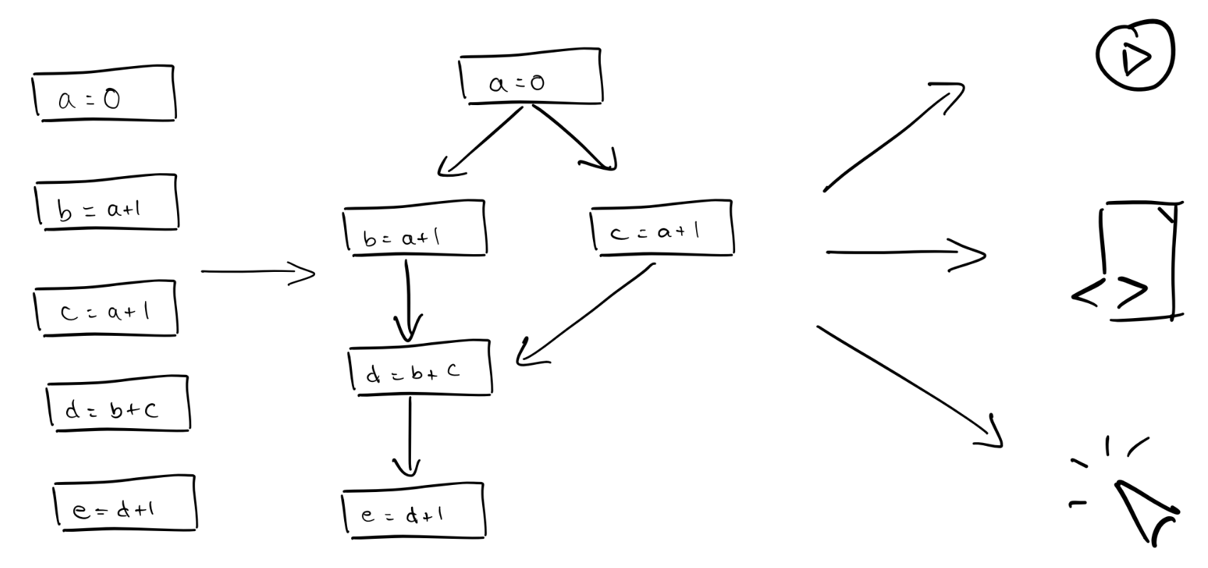
A notebook is shown on the left, and its representation as a dataflow graph is in the middle. On the right are three ways the graph can be executed: as a reactive notebook, in which you can run individual cells; as a script; and as a web app.
The dataflow graph is an intermediate representation for three different ways of running your code:
As a reactive notebook. When you run a cell, marimo uses the dataflow graph to determine which other cells need to run to keep code and outputs in sync. marimo can either run these cells for you automatically or mark them as stale (your choice). This is called reactive execution. Reactivity dramatically speeds up experimentation while also giving you guarantees on state.
As a Python script. Notebooks are stored as Python files in which each
cell is a function. Running python notebook.py runs your cells in a
topologically sorted order.
As an interactive web app. Use marimo run notebook.py from the command-line
to serve your notebook as a web app, with code hidden. Interactions with
UI elements trigger reactive execution of dependent cells — no callbacks
required.
In all three cases, the dataflow graph determines the cell execution order, ensuring that your program’s semantics remain the same.
A contract between marimo and the developer
marimo imposes a few constraints on your code to ensure that your notebook is a directed acyclic graph (DAG).
- No cycles
- No variable redefinitions across cells
These constraints have a small learning curve. But accept these simple-to-understand constraints — sign this contract — and you get many benefits:
- batteries-included: replaces
jupyter,streamlit,jupytext,ipywidgets,papermill, and more - reactive: run a cell, and marimo reactively runs all dependent cells or marks them as stale
- interactive: bind sliders, tables, plots, and more to Python — no callbacks required
- git-friendly: stored as
.pyfiles - designed for data: query dataframes, databases, warehouses, or lakehouses with SQL, filter and search dataframes
- AI-native: generate cells with AI tailored for data work
- reproducible: no hidden state, deterministic execution, built-in package management
- executable: execute as a Python script, parameterized by CLI args
- shareable: deploy as an interactive web app or slides, run in the browser via WASM
- reusable: import functions and classes from one notebook to another
- testable: run pytest on notebooks
- a modern editor: GitHub Copilot, AI assistants, vim keybindings, variable explorer, and more
Plus, you may find that you end up writing better code.
Why marimo does not track mutations
We opted for static construction, based only on variable definitions and references, for two reasons:
- it makes the dataflow structure easy for developers to understand;
- it’s possible for us to implement with 100% correctness.
In contrast, runtime tracing of mutations (such as a list append) would cover more control dependencies, but never all. It would be fundamentally incorrect, stranding developers in an uncanny valley with steep usability cliffs in which they wouldn’t be able to predict how and when their cells would run.
How marimo uses the dataflow graph
Reactive execution
Reactive execution is based on a single runtime rule:
When a cell is run, all other cells that reference its definitions (its descendants) are also run; when a cell is deleted or modified, its definitions are removed from kernel memory and its descendants are re-run.
This keeps code and outputs in sync and prevents bugs before they happen, while also enabling rapid data transformations.
It’s also different from how regular notebooks work, and that can take getting used to. For this reason, marimo provides the affordances that make reactive execution more manageable. Below we list some of these affordances, as well as other ways in which marimo’s runtime uses the graph to make developers more productive.
Lazy execution. The reactive runtime can be configured to be lazy, in which case descendants are marked as stale instead of automatically run. A single click (or hotkey combination) can be used to run all stale cells.
Control flow. Raising an exception halts execution of a cell and its descendants;
marimo provides a convenience function for this, mo.stop(predicate). This allows
developers to author notebooks or workflows in which subtrees of cells are only
executed when their preconditions are met.
Granular re-runs for imports. It is common to declare all notebooks in a cell, incrementally adding additional imports as needed; it would be unfortunate if adding these new imports triggered re-runs of cells depending on the already imported modules. For such cases we statically determine the set of modules imported by a cell; descendants of “import-only” cells are filtered based on new imports, preventing unnecessary re-runs.
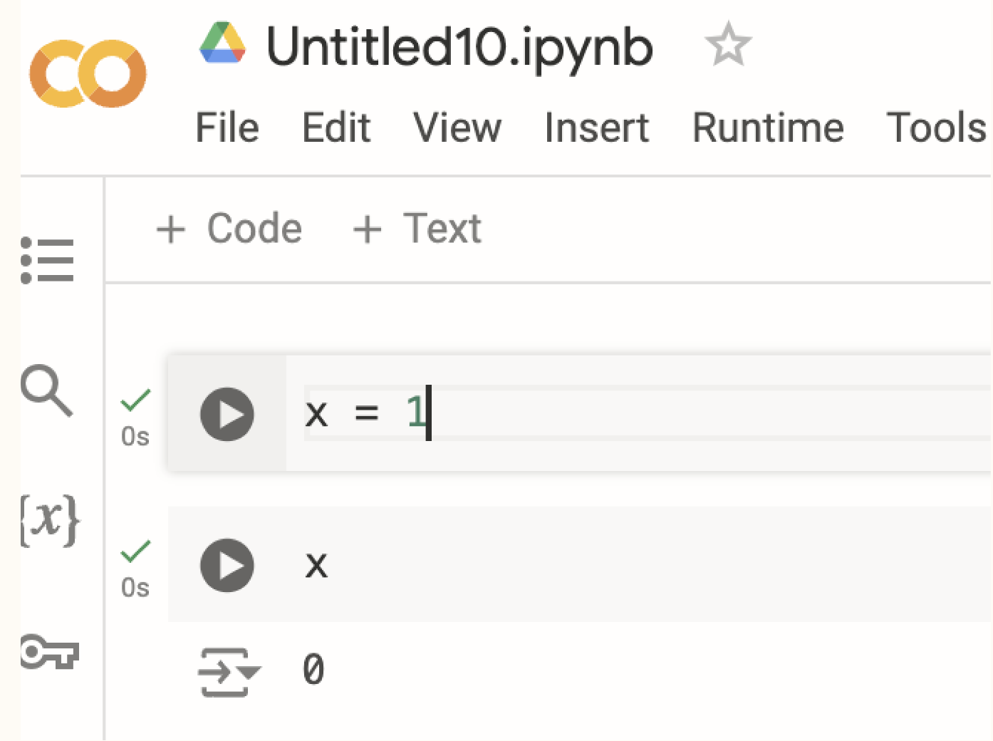
Graceful constraint validation. As mentioned earlier, marimo notebooks have some constraints: a variable cannot be defined in multiple cells, and cycles among cells are not allowed. When a repeated definition is introduced, care is taken to not invalidate previously valid state. In particular, registration of a new cell u should not invalidate
an existing cell v, unless there is a path from u to v.
If you have three cells, run incrementally:
x = 0x# The third cell triggers a multiple definition error, without invalidating the first two cells.
Local variables. To make it easier to adapt to marimo’s constraint, we introduce the following rule: variables prefixed with an underscore are made local to a cell, and so their name can be reused in multiple cells
for _i in range(k): ...This also allows for anonymous scopes, which are a convenient way to avoid polluting the global scope:
def _():
    x = ...
Local variables are implemented by name-mangling while walking the AST and forming the graph.
Module hot-reloading.
marimo comes with an advanced module autoreloader that takes advantage of the dataflow graph.
- On module change, the cells that use modified modules (determined statically, by referring to the graph) are marked stale.
- Modules that depend on these modified modules also marked stale.
- This allows us to know exactly which cells need to be re-run (unlike IPython’s
autoreloadextension).
SQL embedding.
SQL is also supported through an embedding in Python:
- We parse a dataflow graph on SQL, analogous to Python, by specializing
Python AST visitor’s analysis of
Callnodes. - Python and SQL graphs are joined based on return value and referenced variables.
As an example,

is translated to
mo.sql(
f'''
SELECT * FROM df WHERE b < {{max_b_value}}
'''
)
which is subject to static analysis.
Composition. marimo allows for composition of notebooks, implemented by
nesting graphs, each with its own runtime. UIElement interactions and RPCs
are routed through this graph stack.
Caching. Because functools.cache invalidated on cell re-run, marimo comes
with its own caching utilities. import marimo as mo to get …
mo.cache, analogous but keyed on ancestor source and primitive reference values:
- Function code hash
- Content addressed hash (primitive references)
- Execution path hash (ancestor source)
mo.persistent_cacheallows disk caching (local or remote)
Mutable state. marimo encourages functional code and discourages mutations. For advanced users, we provide React-like state setters and getters provide an escape hatch for mutable state (though we discourage this practice, and recommend implementing custom widgets with anywidget instead).
get_state, set_state = mo.state(0)A call to set_state registers a pending state update with the runtime:
set_state(1)When cells have finished executing, any cell with a reference to a getter of a pending state update is marked for execution:
get_state()Interactive elements
The dataflow graph makes it possible for marimo to provide a reactive experience for working with UI elements, no callbacks required. Binding UI elements to global variables connects them to marimo’s runtime.
Interacting with a UI element marks for execution all
cells that refer to its bound variable but don’t define it. In our implementation,
on interaction, the runtime searches globals for matching UIElement objects,
does a lookup to find the bound variables’ defining cells, then triggers reactive
execution.
Scripts
Script execution. marimo stores notebooks as pure Python files, with each cell stored as a function.
import marimo

app = marimo.App()

@app.cell
def _():
    x = 0
    return x

@app.cell
def _(x):
    y = x + 1
    print(y)
    return

if __name__ == "__main__":
    app.run()
Running python my_notebook.py registers the cells with an internal dataflow
graph and runs them in a topologically sorted order.
Reuse as modules.
Any cell that defines a “pure” (no variable references except for those from a special setupcell or other pure functions) function is saved as top-level symbols. Determining which functions are pure requires studying the graph. For example:
import marimo

app = marimo.App()

with app.setup():
   import numpy as np

@app.function
def mean(x: np.ndarray):
    return np.mean(x)

@app.cell
def _():
    print(mean(np.random.randn(2,2)))
    return

if __name__ == "__main__":
    app.run()
Allowing you to write, in another Python file or notebook:
from my_notebook import meanConverting Jupyter notebooks to marimo notebooks. marimo has a built-in
converter from Jupyter notebooks to marimo notebooks (marimo convert at the
command-line), which fixes violated constraints such as multiple definitions.
We extended our AST visitor to transform multiple definitions with static
single assignment:
a = 0aa = a + 1ais remapped to
a = 0aa_1 = a + 1a_1Apps
marimo notebooks can be run as data apps with the command-line: marimo run my_notebook.py, which hides the notebook code by default. Unlike other data
app frameworks, marimo uses the DAG to ensure a minimal set of cells run on UI
element interactions.
Implementation
Representing a notebook as a dataflow graph requires parsing each cell into an abstract syntax tree (AST), then applying semantic analysis to wire up the graph.
Parsing
Parsing means converting user code into an AST. In Python, this involves using
the builtin ast module. For example, the code
b = a + 1is represented by the tree
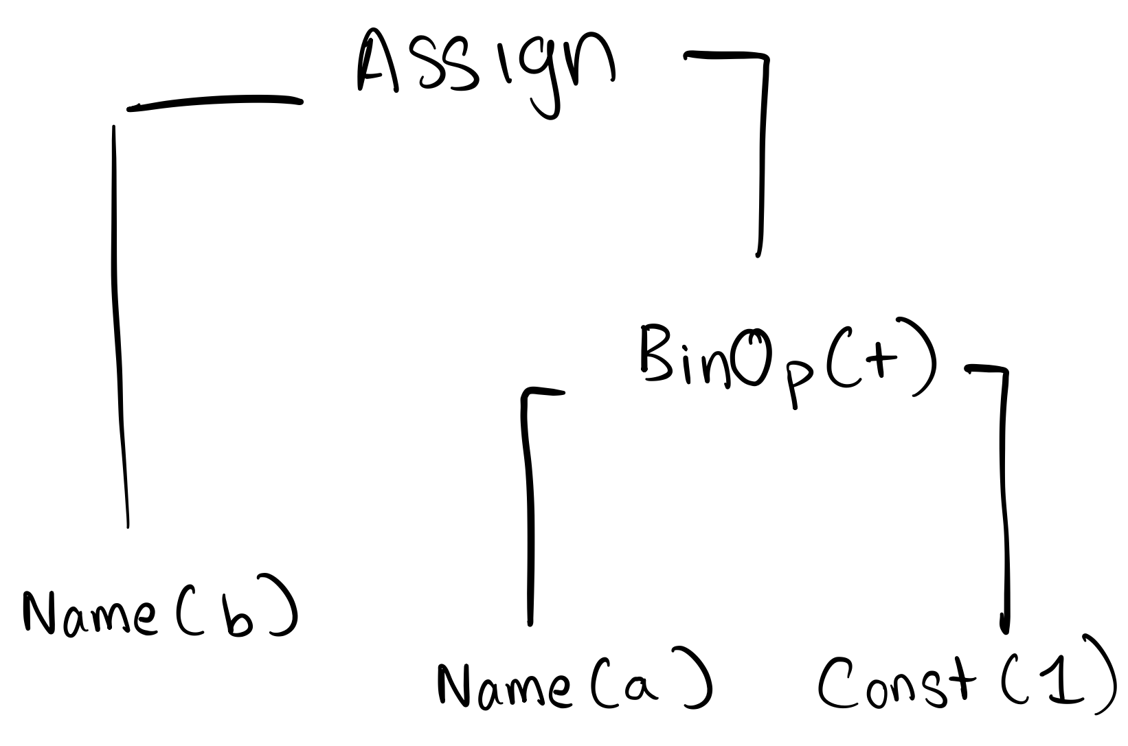
In Python,
import ast

ast.dump(ast.parse("b = a + 1"), indent=4)
yields
Module(
    body=[
        Assign(
            targets=[
                Name(id='b', ctx=Store())
            ],
            value=BinOp(
                left=Name(id='a', ctx=Load()),
                op=Add(),
                right=Constant(value=1)
            )
        )
    ]
)
Semantic analysis
Semantic analysis takes the abstract syntax trees produced in parsing (one for each cell), and makes sense of them:
- We walk the tree to find variables the cell defines, refers to (but doesn’t define), and deletes;
- we construct the graph based on cells’ definitions and references;
- we check whether graph constraints are satisfied.
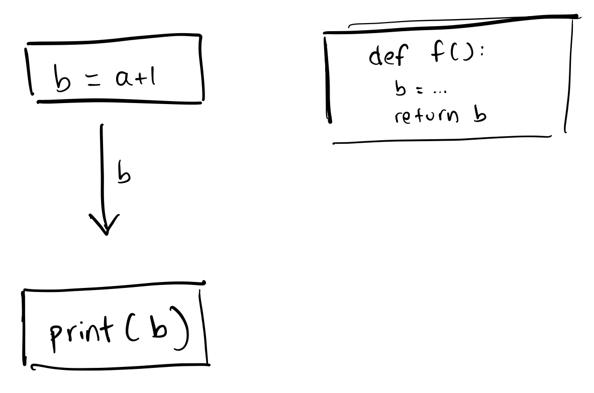
As an example, the sequence of cells
b = a + 1print(b)def f():
b = ...
return bis after analysis formed into the following graph. Notice that the variable b in f is recognized
as local to the cell, since it is defined in a function’s scope.
Variable scope resolution
Determining which variables are definitions and references, and which are local to a cell, is called variable scope resolution:
- Variables are visible in scopes: these are sets of names valid in a specific region.
- Scopes can be nested; inner scopes can access parent scopes’ variables, but not vice versa.
- A cell’s definitions are the variable declarations in global scope.
- A cell’s references are variable load or deletes in any scope that have not been defined in a parent scope.
- Resolving references involves maintaining symbol tables in a stack of scopes.
Example. Consider this code:
def f(d):
    return b + c + d
b = dThe cell defining f references b, c, but not d, since d is shadowed by the function argument.
The cell defining b references d.
Conclusion
marimo’s rapid adoption indicates that developers are willing to sign our social contract. And even though dataflow notebooks may feel new to developers at first, they quickly become accustomed to it.
Statically constructing a dataflow graph gives us enough information to make notebooks reactive, reproducible, and reusable, while still being simple enough that you can understand what’s happening. And because it’s based on static analysis of regular Python code, you get all the benefits of working in Python: compatibility with LLMs and Python tooling, testing, version control, everything you’d expect from a real programming language.
What we ended up with is something that feels like an extremely interactive notebook when you’re developing, works like a script when you need to run it in production, and becomes an app when you want to share it with others.
Join the marimo community
If you're interested in helping shape marimo's future, here are some ways you can get involved: