Signal Decomposition
by marimo team
Breaking a complex signal into the sum of simpler interpretable components.
About this notebook
This notebook is a two-part tutorial on signal decomposition, which splits a time series into a sum of simpler component signals. The tutorial follows the book "Signal Decomposition Using Masked Proximal Operators" by Bennet Meyers and Stephen Boyd. It computes each decomposition with the signal-decomp library and plots the results with matplotlib.
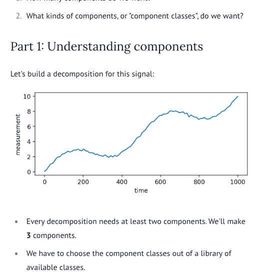
Part 1 asks you to decompose a synthetic signal made from a line plus a sine wave. Radio buttons choose the class of each component: trend line, periodic, or piecewise constant. The notebook plots the decomposition after each choice and explains the selected class in a callout. marimo state tracks which classes you tried, and a button adds a third component when two are not enough. When you combine the trend-line and periodic classes, a success message unlocks part 2.
Part 2 offers a dropdown of real-world and synthetic signals, including atmospheric CO2 from the Mauna Loa Observatory, and accepts a CSV file that you upload. Buttons add or remove components, dropdowns select the class of each one, and generated controls set its parameters. The first component always represents the noise. The notebook computes a decomposition once you choose a noise component and at least one more component, then plots every component and the denoised signal. A reference dropdown explains every component class. At run time the notebook downloads its helper modules from the gallery-examples repository.