Simpson's Paradox with PyMC
by marimo team
Explore Simpson's paradox with Bayesian modeling, showing how confounding variables can reverse observed trends.
About this notebook
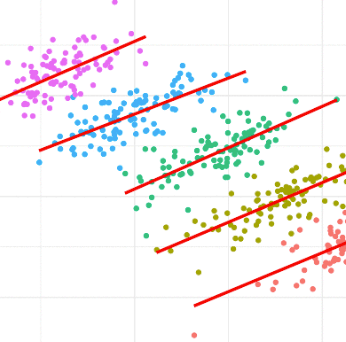
This notebook shows Simpson's paradox with Bayesian regression. The paradox can appear when a relationship inside each group reverses after you combine all groups. The notebook builds its own dataset with NumPy. It makes five groups with 20 observations each. Inside each group the slope between x and y is negative. Across all groups combined the slope looks positive. The models use PyMC. The plots use Matplotlib, seaborn, and ArviZ. The notebook adapts a PyMC docs example by Benjamin T. Vincent.
The notebook fits three models to the same data. It draws each model as a causal DAG with graphviz. For each model it shows trace plots, scatter plots, and posterior bands from ArviZ. A parameter space plot shows the joint posterior of the slope and intercept. Model 1 pools all data and suggests a positive slope. Models 2 and 3 add the group variable and suggest negative slopes. The notebook cells run in order and show static plots. It does not include interactive widgets.
The three models differ in structure. Model 1 is a pooled regression with one intercept and one slope. Model 2 is an unpooled model with a separate intercept and slope for each group. Model 3 is a hierarchical model where the group parameters come from a population distribution. Each model uses Normal and Gamma priors. PyMC samples the posterior with pm.sample and a fixed random seed. A predict function draws posterior predictive samples at new x values.