Smoothed Gradient Descent
by marimo team
Visualize gradient descent with momentum and smoothing techniques
About this notebook
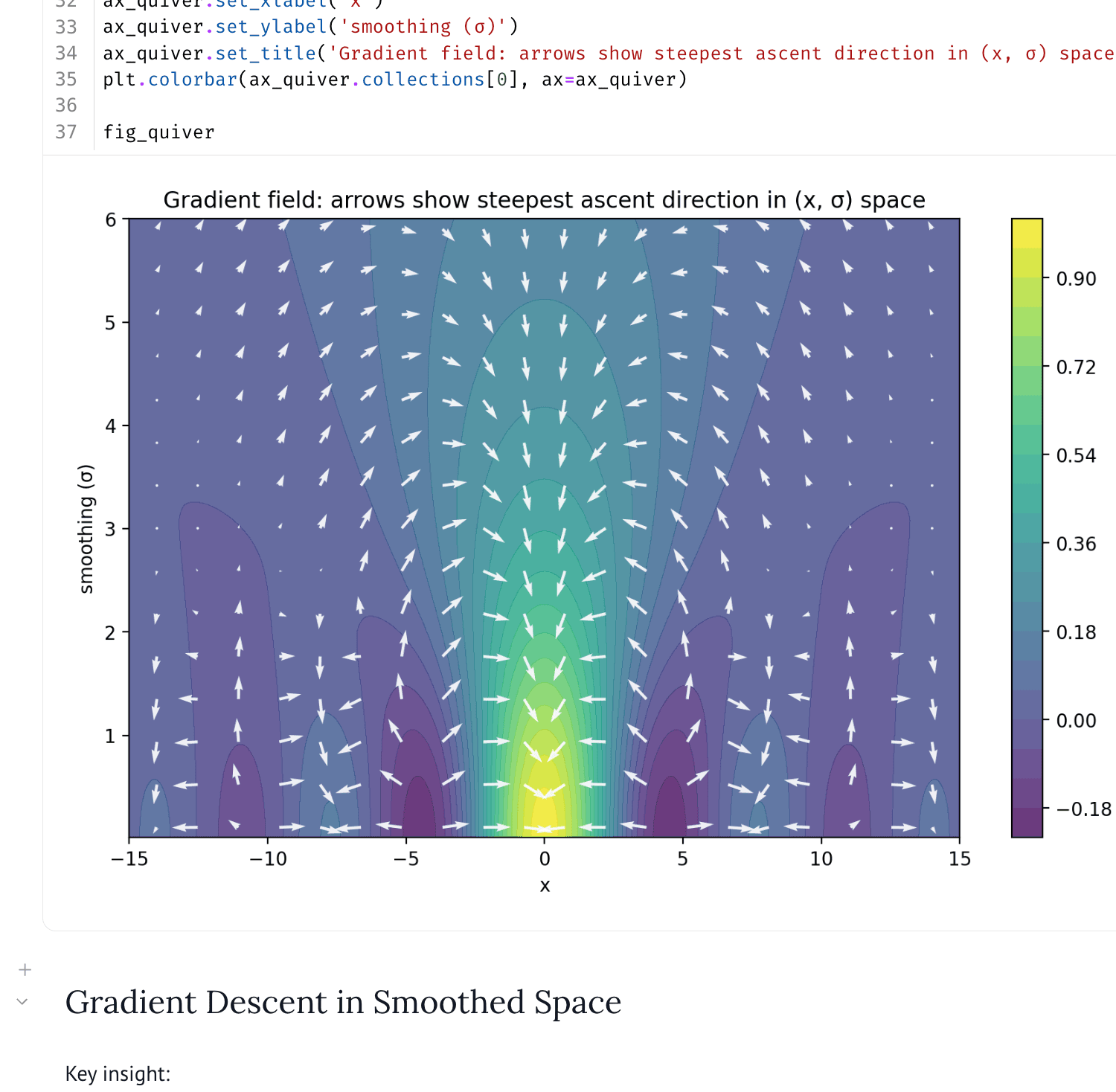
This notebook shows how Gaussian smoothing helps optimise hard functions. It uses two example functions. The first is the sinc function. The second is a floor function that combines sinc and a sine term, so it is non- differentiable. Both functions have many local peaks. The notebook builds on NumPy, SciPy, and matplotlib inside marimo. It adds a smoothing parameter to turn each one-dimensional problem into a two-dimensional landscape g(x, s). At high smoothing the landscape is smooth. At zero smoothing it matches the original function.
Two sliders set the position x and the smoothing sigma. When you move them, the left plot draws the function, the Gaussian, and their product. The green shaded area equals the integral. The right plot marks that same value as a pixel on the heatmap. A dropdown chooses the sinc or floor function. More sliders set the start point, the start smoothing, and the step count. The final chart then compares three optimisation paths on the chosen landscape.
The smoothed value comes from a Gaussian-weighted integral. The code integrates over plus or minus four sigma with the trapezoid rule. It builds each landscape on a grid of 1000 x values and 40 smoothing values. This step may take a moment. The three compared methods are gradient descent on g, evolution strategies on f, and evolution strategies on g. Each method follows the smoothing dimension with a small bias toward lower smoothing.